How does torch.compile speed up a transformer?
torch.compile is now a go-to tool for optimizing performance of PyTorch models, but it's often treated a black box. Fortunately, it's easy to see what sort of optimizations it makes. Let's study some of these by looking at the use case of a vision transformer (ViT).
Anatomy of a ViT
We'll be looking at the ViT-g/14 architecture used in DINOv2 1. This model has a few more bells and whistles compared to a vanilla ViT which will offer torch.compile more opportunities to illustrate some optimizations. The model architecture parameters are described below:
| Parameter | Value |
|---|---|
| Embedding dimension | 1536 |
| No. attention heads | 24 |
| No. layers | 40 |
| MLP layer type | SwiGLU |
| LayerScale | True |
| No. paramters | 1B |
This model can be instantiated by doing:
import timm

# can set pretrained=False if you don't want to download the weights.
# pretrained vs. random weights won't make a difference for profiling
model = timm.create_model('vit_giant_patch14_dinov2.lvd142m', pretrained=True)
model = model.eval().half().cuda()
Let's understand the computation graph of this architecture before looking at optimizations. Below is an image illustrating the flow of operations for this model (imagine though it's a 1 layer ViT instead of 40 layers). Read from bottom to top.
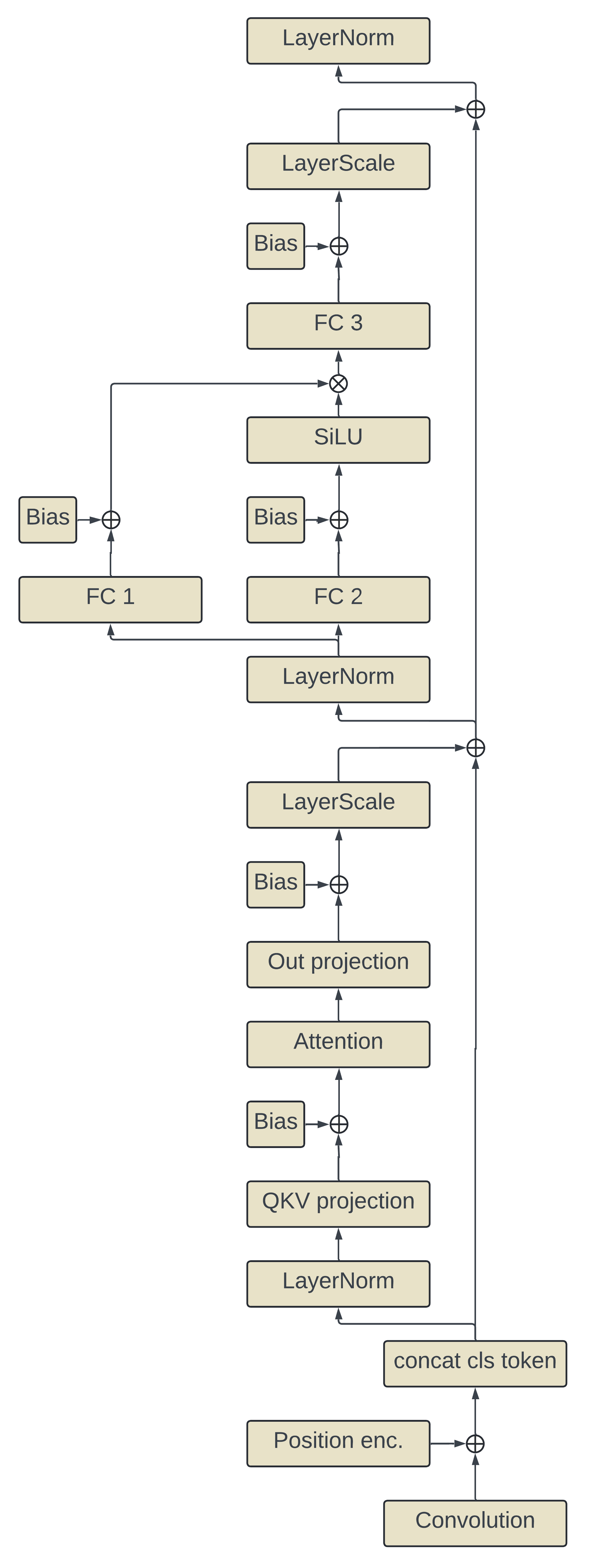
The first layer is implemented as a convolutional layer with a kernel size of 14x14 and stride of 14x14. This is the patch embedding layer that projects a 14x14x3 patch of pixels into the 1536 embedding dimensions. Learned positional encodings are then added to the patch embeddings, followed by prepending the learned cls token to the sequence. This model is a modern pre-LN transformer meaning the layer normalization is done on the inputs to the layers. After the layer norm, the sequence is projected into queries, key, and values and a bias is added. Scaled dot-product attention is applied and followed by the attention layer output projection and addition of biases. Unlike a vanilla ViT, a layer scale, a multiplicative operation, is applied before the attention layer's output is summed with the residual. The sequence then goes through the layer norm of the MLP block followed by two parallel linear layers plus biases (implemented as one big matmul though). The output of one of these linear layers has the SiLU activation applied to it and then that is used to multiplicatively gate the output of the other linear layer. This product then goes through one more linear layer with biases before another layer scale is applied followed by addition with the residual and a final layer norm.
Eager mode kernels
Now that we've defined the computation graph we can look at how PyTorch would normally execute these operations in the default eager mode. One way of investigating this is to use a CUDA profiling tool like Nvidia Nsight Systems. If we zoom into a single ViT layer we can see the kernels that PyTorch dispatches to for each operation (best viewed if the image is opened in a new tab, sorry).
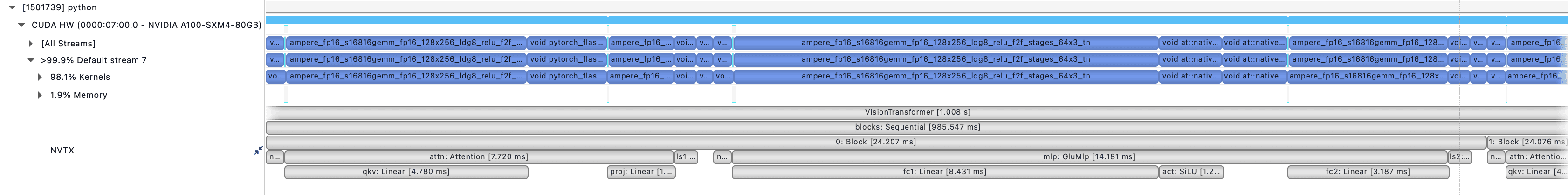
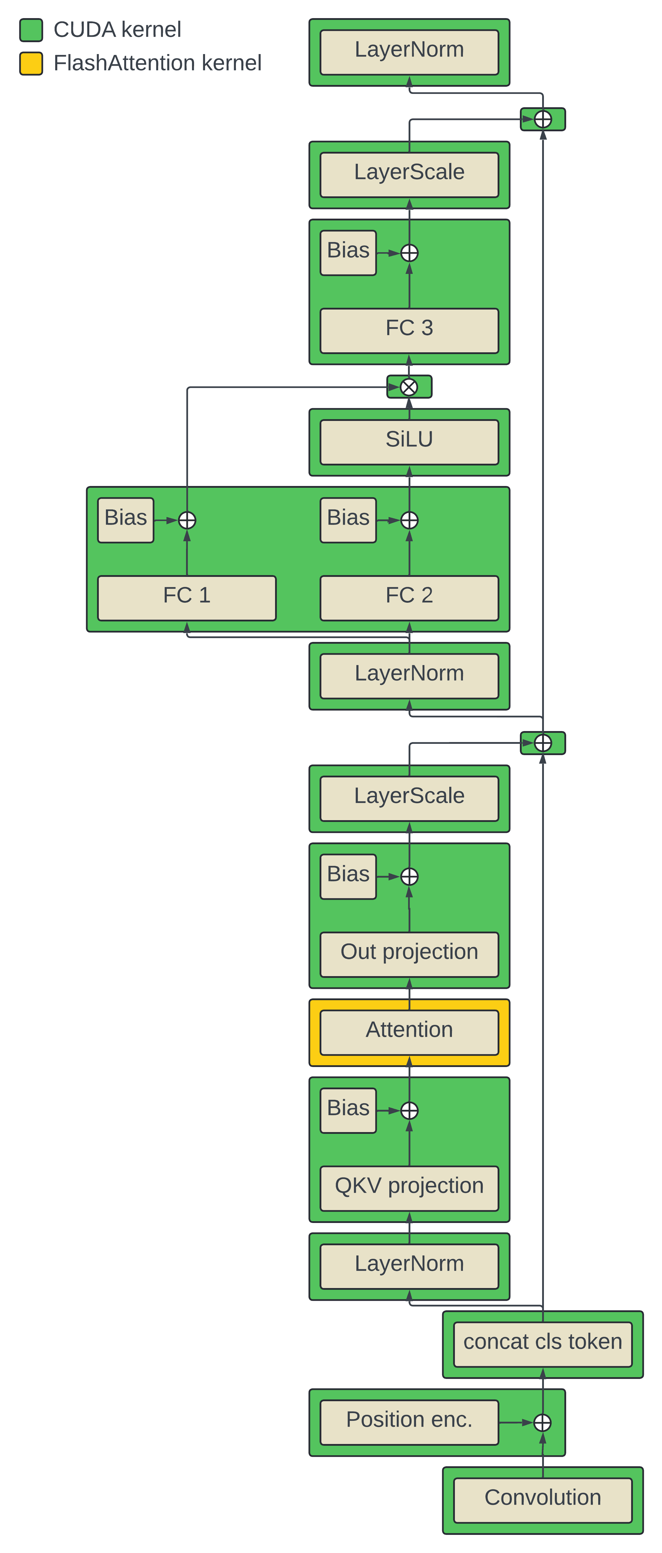
I've added NVTX annotations to try and make it easier to see the mapping of the operations in the computation graph illustration to the actual kernels selected by PyTorch. For all the operations in our graph illustration, there is a 1-to-1 mapping to a kernel invocation with the exception of the linear layer biases which are added in their associated matmul kernel. The updated graph below illustrates this by color coding each operation. I refer to every kernel used here by eager mode generically as "CUDA kernels" except for the FlashAttention kernel (though this distinction is not particularly meaningful for this topic).
The important part here is that PyTorch only dispatches operations to a set pre-written CUDA kernels that it can choose from. This is useful to allow for eager execution where we can write arbitrary graphs of PyTorch operations and then all 2 PyTorch has to do is invoke the associated kernels. This means that those kernels have to be written in an a rather atomic and isolated manner so that they can be plugged into any order of operations. In other words, the kernels are written without knowing anything about the preceding or suceding operations. This generality comes at the cost of performance because it prevents using kernels that are optimized for the specific sequences of operations in our computation graph.
Kernel fusion
To understand how kernel-level optimizations can be made when considering a specific sequence of operations, let's first cover the high level basics of how GPUs and CUDA kernels work.
GPUs have what is called global memory which is the memory you'll usually be familiar with when reading the specs of the card. The A100 GPUs have either 40GB or 80GB of global memory, H100s have 80GB, a 4090 has 24GB, etc. This global memory is made up of high bandwidth (HBM) DRAM and is where all our model parameters, activations, gradients, optimizer states, and all other on-device tensors are stored. In order to do computation with any of these tensors, they need to be read from the global memory onto the chip where computation actually takes place. This data is read into the much smaller but much faster on-chip memory/registers to be the used by the logic cores. The output of the computation then needs to be written back out to global memory.
A CUDA kernel takes care of these operations and the very basic pattern of a kernel is:
read x
compute y = f(x)
write y
An issue here is that accessing data from global memory can be quite slow relative to the speed of the actual computation. This depends on the specs of our GPU like the memory bandwidth and chip speeds and also the nature of the computation, i.e. the ratio of operations to bytes accessed (known as arithmetic intensity). Operations like matmuls can be well-optimized to have a high enough ratio of ops:bytes to be considered "compute-bound", meaning the bottleneck becomes the speed of the chip doing the calculations. Other operations like pointwise adds, multiplications, activation functions, etc. naturally will have lower ops:byte ratios where they are considered "memory bandwidth bound" meaning the bottleneck is the speed of data transfer between the global memory and the chip.
If we look at the color-coded computation graph from before we know now that there are global memory accesses going on in each of these kernels. Most of these accesses seem redundant though and could be slowing things down. Why spend time loading data to do a small operation on it like adding with the residual just to load that output again to do layer norm?
The idea of kernel fusion is to combine these sucessive operations to eliminate unnecessary memory accesses and thus increase the number of operations done per byte of data read. Before kernel fusion we might have two kernels doing:
def kernel_1(x):
  read(x)
  y = f(x)
  write(y)

def kernel_2(y):
  read(y)
  z = g(y)
  write(z)
Fusing these kernels would produce a single kernel that executes:
def fused_kernel(x):
  read(x)
  z = g(f(x))
  write(z)
This reduced the memory accesses by half and increased the arithmetic intensity of this sequence of operations.
torch.compile kernels
Kernel fusion is a large part of how torch.compile optimizes models. It achieves this by inspecting the computation graph of a model and writing custom Triton 3 kernels that fuses operations. The ability to codegen specific kernels at compile time is a large advantage over the eager mode execution strategy. torch.compile makes it easy to inspect generated Triton code by setting the env var TORCH_COMPILE_DEBUG=1. This will save the Triton code to a Python file in a directory named torch_compile_debug/. We can run this with:
import os

import timm
import torch

# can set pretrained=False if you don't want to download the weights. pretrained vs. random weights won't make a difference for just profiling speed
model = timm.create_model('vit_giant_patch14_dinov2.lvd142m', pretrained=True)
model = model.eval().half().cuda()

os.environ['TORCH_COMPILE_DEBUG'] = '1'
model = torch.compile(model, fullgraph=True)

x = torch.randn(256, 3, 224, 224).half()

with torch.inference_mode():
  out = model(x)
By inspecting the generated kernels (see Appendix A) we can figure out which regions of the computation it decides to fuse. Based on the benefits of fusion described above we can predict that sequences of operations with low arithmetic intensity will be good candidates for torch.compile to optimize. The illustration below describes the regions that torch.compile wrote custom kernels for as well as operations that still dispatched CUDA kernels:
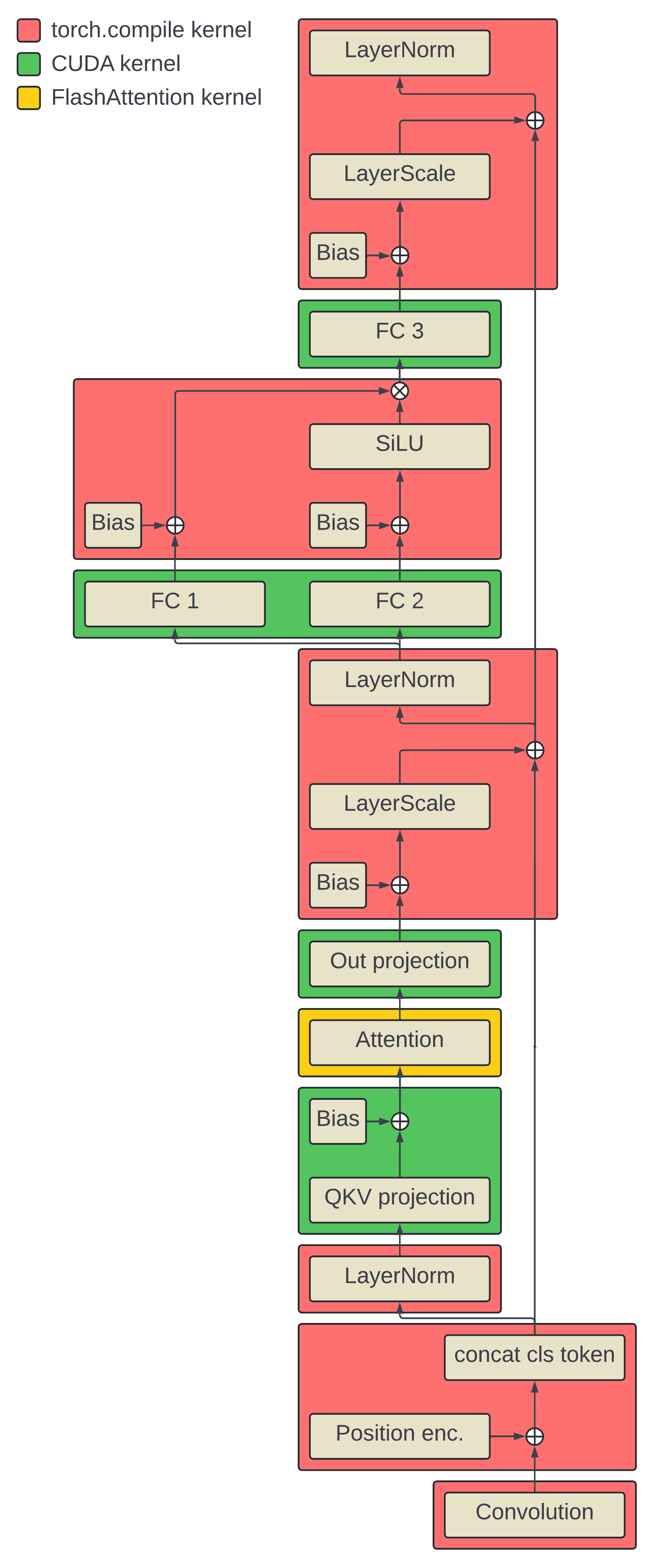
All the linear layers and attention still dispatch to CUDA/FlashAttention kernels respectively because these are already highly optimized implementations. torch.compile wrote a Triton implementation for the patch embed convolutional layer, fused the addition of position encodings with the concatenation of the cls token, and generated a fused layer norm implementation. Interestingly, it also fused several sequences of low arithmetic intensity ops as predicted. Let's take a closer look at these.
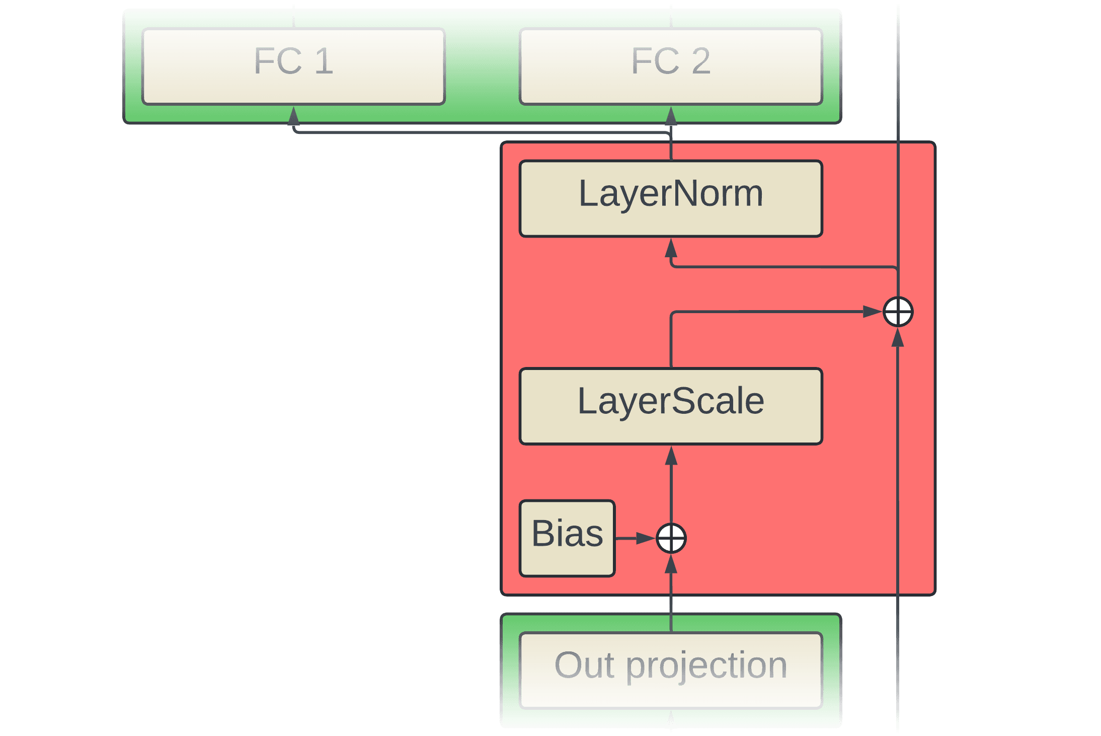
The region above gets fused into one kernel. The addition of the bias, layer scale multiplication, addition with the residual, and layer norm are all memory bound operations by themselves but by fusing them there is much less read/writes. Below is some high-level pseudocode of each of the kernels for these operations pre-fusion:
def add_bias_kernel(x_ptr, bias_ptr, out_ptr):
  # Add preceding linear layer bias
  x = read(x_ptr)
  bias = read(bias_ptr)

  x = x + bias

  write(out_ptr, x)
Where *_ptr are pointers to tensors in global memory. add_bias_kernel reads the input sequence x (shape: batch x 257 x 1536) and bias vector (shape: 1536) and does pointwise addition and writes out the result.
def mul_layer_scale_kernel(x_ptr, gamma_ptr, out_ptr):
  # Multiply layer scale gamma
  x = read(x_ptr)
  gamma = read(x_ptr)

  x = x * gamma

  write(out_ptr, x)
mul_layer_scale_kernel reads in the input sequence x and the learned layer scale gamma vector (shape: 1536) and does pointwise multiplication and writes out the results.
def add_residual_kernel(x_ptr, res_ptr):
  # Add residual
  x = read(x_ptr)
  res = read(res_ptr)

  x = x + res

  write(out_ptr, x)
add_residual_kernel looks similar to add_bias_kernel and does the same amount of FLOPs, but the memroy bandwidth pressure is higher since, in addition to reading x, we'd also be reading the residual vectors res (shape: batch x 257 x 1536) instead of a single bias vector (shape: 1536).
def layer_norm_kernel(x_ptr, scale_ptr, bias_ptr, out_ptr):
  # Layer norm
  x = read(x_ptr)
  scale = read(scale_ptr)
  bias = read(bias_ptr)

  mean = mean(x, dim=-1)
  var = mean((x - mean)**2, dim=-1)
  rstd = (var + 1e-5) ** -0.5
  norm = (x - mean) * rstd
  out = norm * scale + bias

  write(out_ptr, out)
layer_norm_kernel reads the input sequence x (shape: batch x 257 x 1536) along with the scale vector (shape: 1536) and bias vector (shape: 1536), applies layer normalization, and writes out the result.
As mentioned earlier, each kernel does it's own read/writes despite doing relatively few FLOPs. The pseudocode below displays how these kernels get fused by torch.compile.
def fused_add_mul_add_ln_kernel(x_ptr, bias_ptr, gamma_ptr, res_ptr, scale_ptr, ln_bias_ptr, out_ptr):
  # Add preceding linear layer bias
  x = read(x_ptr)
  bias = read(bias_ptr)

  x = x + bias

  # Multiply layer scale gamma
  gamma = read(x_ptr)

  x = x * gamma

  # Add residual
  res = read(res_ptr)

  x = x + res

  # Layer norm
  scale = read(scale_ptr)
  bias = read(bias_ptr)

  mean = mean(x, dim=-1)
  var = mean((x - mean)**2, dim=-1)
  rstd = (var + 1e-5) ** -0.5
  norm = (x - mean) * rstd
  out = norm * scale + bias

  write(out_ptr, x)

# one kernel invocation
fused_add_mul_add_ln_kernel(x, bias, gamma, res, scale, ln_bias, out)
Now instead of redundantly reading the input (x) before each operation, it's only read once. Also, the intermediate outputs don't get written back to global memory anymore, only the final output gets stored.
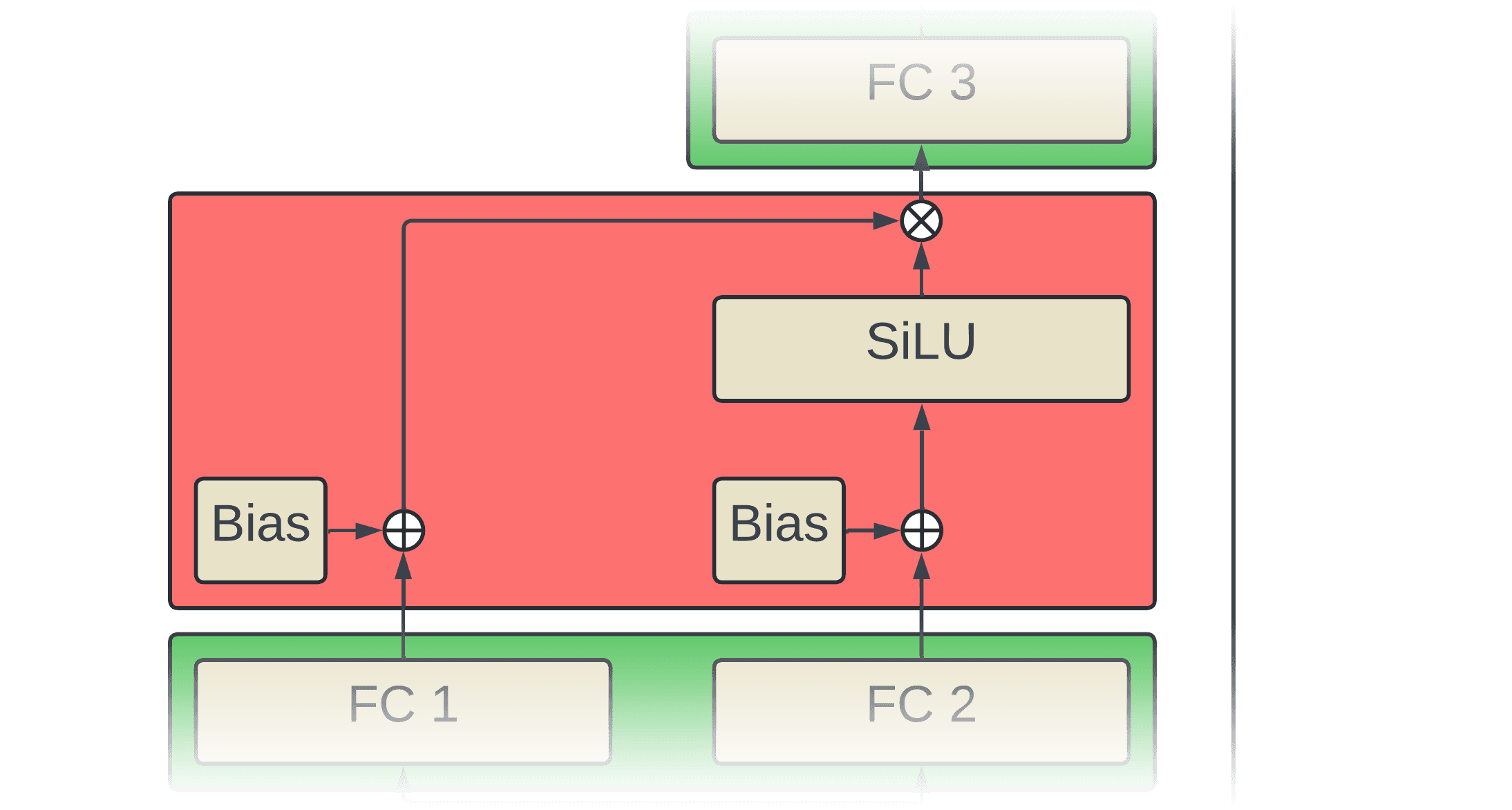
Another region of the graph that gets fused are the first MLP layer biases, SiLU, and gating multiplication.
Let's look at the pre-fusion pseudocode:
def add_bias_kernel(x_ptr, bias_ptr, out_ptr):
  # Add preceding linear layer bias
  x = read(x_ptr)
  bias = read(bias_ptr)

  x = x + bias

  write(out_ptr, x)
This is the same as add_bias_kernel that was shown earlier except at this point we read the outputs and bias vector of FC 1 and FC 2 which when packed together are shapes batch x 257 x 8192 and 8192 respectively.
def silu_kernel(x_ptr, out_ptr):
  # Apply SiLU activation
  x = read(x_ptr)

  x = x * sigmoid(x)

  write(out_ptr, x)
silu_kernel reads the output of just FC2 (shape: batch x 257 x 4096) applies the sigmoid function to it and does element-wise multiplication as a gating function on the input and then writes out the result.
def mul_kernel(a_ptr, b_ptr, out_ptr):
  # Multiply
  a = read(a_ptr)
  b = read(b_ptr)

  x = a * b

  write(out_ptr, x)
mul_kernel reads the output of FC 1 + bias (shape: batch x 257 x 4096) and the output of the SiLU (shape: batch x 257 x 4096) and does element-wise multiplication between them and write out the result.
Similar to the add -> mul -> add -> layer norm region, each kernel is doing redundant read/writes and few FLOPs. The fused kernel below only needs to read the inputs and write the output once:
def fused_add_silu_mul_kernel(x_ptr, bias_ptr, out_ptr):
  # Add preceding linear layer bias
  x = read(x_ptr)
  bias = read(bias_ptr)

  x = x + bias

  x1, x2 = x.chunk(2, dim=-1)

  # Apply SiLU activation
  x1 = x1 * sigmoid(x1)

  # Multiply
  x = x1 * x2

  write(out_ptr, x)
Conclusion
So how much does all this kernel fusion speed up inference? On an A100 80GB card, the eager inference time for a batch size of 256 224x224 images clocks in at ~1000 ms and ater applying torch.compile that time comes down to ~870 ms. This article doesn't paint the full picture of what torch.compile does and there's a bit more than just kernel fusion that allows it make optimizations, but that's beyond the scope of this post.
Even though torch.compile has become a crucial component to running efficient PyTorch models, there can still be room for optimizations that it isn't quite able to find for itself 4. In the case of this ViT architecture, one example is that the LayerScale weights (gamma) can be multiplied into the weights and biases of the linear layer before it in order to completely eliminate the multiplication op of LayerScale while maintaining mathematical equivalance (see Appendix B).
Citation
@article{casson2024compilevit,
  author={Adam Casson},
  title={How does torch.compile speed up a transformer?},
  year={2024},
  url={https://adamcasson.com/posts/torch-compile-vit}
}
Appendix A: torch.compile generated Triton kernels
A warning to the reader, this is auto-generated code and it's not the most readable.
Convolution (patch embedding)
@triton.jit
def triton_(arg_X, arg_W, out_ptr0):
    KERNEL_H : tl.constexpr = 14
    KERNEL_W : tl.constexpr = 14
    STRIDE_H : tl.constexpr = 14
    STRIDE_W : tl.constexpr = 14
    PADDING_H : tl.constexpr = 0
    PADDING_W : tl.constexpr = 0
    GROUPS : tl.constexpr = 1
    UNROLL : tl.constexpr = False
    ALLOW_TF32 : tl.constexpr = True
    BLOCK_M : tl.constexpr = 256
    BLOCK_N : tl.constexpr = 64
    BLOCK_K : tl.constexpr = 16

    X = arg_X
    W = arg_W

    # Tensor dimensions
    BATCH = 256
    IN_C = 3
    IN_H = 224
    IN_W = 224
    OUT_C = 1536
    OUT_H = 16
    OUT_W = 16

    # Strides:
    stride_xn = 150528
    stride_xc = 50176
    stride_xh = 224
    stride_xw = 1
    stride_wc_out = 588
    stride_wc_in = 196
    stride_wh = 14
    stride_ww = 1

    nhw = tl.program_id(0) * BLOCK_M + tl.arange(0, BLOCK_M)
    idx_y_w = nhw % OUT_W
    nh = nhw // OUT_W
    idx_y_h = nh % OUT_H
    idx_n = nh // OUT_H
    idx_y_c = tl.program_id(1) * BLOCK_N + tl.arange(0, BLOCK_N)


    group = 0
    GROUP_IN_C = IN_C
    GROUP_OUT_C = OUT_C


    x_base = X + (group * stride_xc * GROUP_IN_C + idx_n * stride_xn)[:, None]
    w_base = (
        W + (group * stride_wc_out * GROUP_OUT_C + idx_y_c * stride_wc_out)[None, :]
    )

    acc = tl.zeros((BLOCK_M, BLOCK_N), dtype=tl.float32)


    # Could be simplified, but slightly slower:
    # for i in range(KERNEL_H):
    #     for j in range(KERNEL_W):
    #         for k in range(0, GROUP_IN_C, BLOCK_K):
    BLOCK_K_COUNT = (GROUP_IN_C + BLOCK_K - 1) // BLOCK_K
    for ijk in range(KERNEL_H * KERNEL_W * BLOCK_K_COUNT):
        k = (ijk % BLOCK_K_COUNT) * BLOCK_K
        ij = ijk // BLOCK_K_COUNT
        i = ij // KERNEL_W
        j = ij % KERNEL_W

        idx_x_h = i - PADDING_H + idx_y_h * STRIDE_H
        idx_x_w = j - PADDING_W + idx_y_w * STRIDE_W
        idx_x_c = tl.arange(0, BLOCK_K) + k

        x_ptrs = x_base + (
            (idx_x_h * stride_xh)[:, None]
            + (idx_x_w * stride_xw)[:, None]
            + (idx_x_c * stride_xc)[None, :]
        )
        mask_x = (
            (idx_n < BATCH)[:, None]
            & (idx_x_h >= 0)[:, None]
            & (idx_x_h < IN_H)[:, None]
            & (idx_x_w >= 0)[:, None]
            & (idx_x_w < IN_W)[:, None]
            & (idx_x_c < GROUP_IN_C)[None, :]
        )
        matrix_x = tl.load(x_ptrs, mask=mask_x, other=0.0)

        w_ptrs = w_base + (
            (idx_x_c * stride_wc_in)[:, None] + (i * stride_wh) + (j * stride_ww)
        )
        mask_w = (idx_x_c[:, None] < GROUP_IN_C) & (idx_y_c[None, :] < GROUP_OUT_C)
        matrix_w = tl.load(w_ptrs, mask=mask_w, other=0.0)
        acc += tl.dot(matrix_x, matrix_w, allow_tf32=ALLOW_TF32)

    mask = (
        (idx_n < BATCH)[:, None]
        & (idx_y_h < OUT_H)[:, None]
        & (idx_y_w < OUT_W)[:, None]
        & (idx_y_c < GROUP_OUT_C)[None, :]
    )
    idx_n = idx_n[:, None]
    idx_c = idx_y_c[None, :] + group * GROUP_OUT_C
    idx_h = idx_y_h[:, None]
    idx_w = idx_y_w[:, None]

    # inductor generates a suffix
    xindex = idx_w + (16*idx_h) + (256*idx_c) + (393216*idx_n)
    tl.store(out_ptr0 + (tl.broadcast_to(xindex, mask.shape)), acc, mask)
Add position embedding and concat cls token
@triton.jit
def triton_(in_ptr0, in_ptr1, in_ptr2, in_ptr3, in_ptr4, out_ptr0, xnumel, XBLOCK : tl.constexpr):
    xnumel = 101056512
    xoffset = tl.program_id(0) * XBLOCK
    xindex = xoffset + tl.arange(0, XBLOCK)[:]
    xmask = xindex < xnumel
    x0 = xindex % 257
    x1 = (xindex // 257) % 1536
    x3 = (xindex // 257)
    x4 = xindex
    tmp0 = x0
    tmp1 = tl.full([1], 0, tl.int64)
    tmp2 = tmp0 >= tmp1
    tmp3 = tl.full([1], 1, tl.int64)
    tmp4 = tmp0 < tmp3
    tmp5 = tl.load(in_ptr0 + (x1), tmp4, eviction_policy='evict_last', other=0.0).to(tl.float32)
    tmp6 = tl.full(tmp5.shape, 0.0, tmp5.dtype)
    tmp7 = tl.where(tmp4, tmp5, tmp6)
    tmp8 = tmp0 >= tmp3
    tmp9 = tl.full([1], 257, tl.int64)
    tmp10 = tmp0 < tmp9
    tmp11 = tl.load(in_ptr1 + ((256*x3) + (((-1) + x0) % 256)), tmp8, eviction_policy='evict_last', other=0.0).to(tl.float32)
    tmp12 = tl.load(in_ptr2 + (x1), tmp8, eviction_policy='evict_last', other=0.0).to(tl.float32)
    tmp13 = tmp11 + tmp12
    tmp14 = tl.full(tmp13.shape, 0.0, tmp13.dtype)
    tmp15 = tl.where(tmp8, tmp13, tmp14)
    tmp16 = tl.where(tmp4, tmp7, tmp15)
    tmp17 = tl.load(in_ptr3 + (x1), tmp4, eviction_policy='evict_last', other=0.0).to(tl.float32)
    tmp18 = tl.full(tmp17.shape, 0.0, tmp17.dtype)
    tmp19 = tl.where(tmp4, tmp17, tmp18)
    tmp20 = tl.load(in_ptr4 + ((256*x1) + (((-1) + x0) % 256)), tmp8, eviction_policy='evict_last', other=0.0)
    tmp21 = tmp20.to(tl.float32)
    tmp22 = tl.full(tmp21.shape, 0.0, tmp21.dtype)
    tmp23 = tl.where(tmp8, tmp21, tmp22)
    tmp24 = tl.where(tmp4, tmp19, tmp23)
    tmp25 = tmp16 + tmp24
    tl.store(out_ptr0 + (x4), tmp25, None)
Layer norm
@triton.jit
def triton_(in_ptr0, in_ptr1, in_ptr2, out_ptr2, xnumel, rnumel, XBLOCK : tl.constexpr, RBLOCK : tl.constexpr):
    xnumel = 65792
    rnumel = 1536
    xoffset = tl.program_id(0) * XBLOCK
    xindex = xoffset + tl.arange(0, XBLOCK)[:, None]
    xmask = xindex < xnumel
    rbase = tl.arange(0, RBLOCK)[None, :]
    x0 = xindex % 257
    x1 = (xindex // 257)
    tmp3_mean = tl.zeros([XBLOCK, RBLOCK], tl.float32)
    tmp3_m2 = tl.zeros([XBLOCK, RBLOCK], tl.float32)
    tmp3_weight = tl.zeros([XBLOCK, RBLOCK], tl.float32)
    x3 = xindex
    for roffset in range(0, rnumel, RBLOCK):
        rindex = roffset + rbase
        rmask = rindex < rnumel
        r2 = rindex
        tmp0 = tl.load(in_ptr0 + (x0 + (257*r2) + (394752*x1)), rmask & xmask, eviction_policy='evict_last', other=0.0).to(tl.float32)
        tmp1 = tmp0.to(tl.float32)
        tmp2 = tl.broadcast_to(tmp1, [XBLOCK, RBLOCK])
        tmp3_mean_next, tmp3_m2_next, tmp3_weight_next = triton_helpers.welford_reduce(
            tmp2, tmp3_mean, tmp3_m2, tmp3_weight,
        )
        tmp3_mean = tl.where(rmask & xmask, tmp3_mean_next, tmp3_mean)
        tmp3_m2 = tl.where(rmask & xmask, tmp3_m2_next, tmp3_m2)
        tmp3_weight = tl.where(rmask & xmask, tmp3_weight_next, tmp3_weight)
    tmp3_tmp, tmp4_tmp, tmp5_tmp = triton_helpers.welford(
        tmp3_mean, tmp3_m2, tmp3_weight, 1
    )
    tmp3 = tmp3_tmp[:, None]
    tmp4 = tmp4_tmp[:, None]
    tmp5 = tmp5_tmp[:, None]
    for roffset in range(0, rnumel, RBLOCK):
        rindex = roffset + rbase
        rmask = rindex < rnumel
        r2 = rindex
        tmp6 = tl.load(in_ptr0 + (x0 + (257*r2) + (394752*x1)), rmask & xmask, eviction_policy='evict_first', other=0.0).to(tl.float32)
        tmp15 = tl.load(in_ptr1 + (r2), rmask, eviction_policy='evict_last', other=0.0).to(tl.float32)
        tmp18 = tl.load(in_ptr2 + (r2), rmask, eviction_policy='evict_last', other=0.0).to(tl.float32)
        tmp7 = tmp6.to(tl.float32)
        tmp8 = tmp7 - tmp3
        tmp9 = 1536.0
        tmp10 = tmp4 / tmp9
        tmp11 = 1e-06
        tmp12 = tmp10 + tmp11
        tmp13 = tl.math.rsqrt(tmp12)
        tmp14 = tmp8 * tmp13
        tmp16 = tmp15.to(tl.float32)
        tmp17 = tmp14 * tmp16
        tmp19 = tmp18.to(tl.float32)
        tmp20 = tmp17 + tmp19
        tmp21 = tmp20.to(tl.float32)
        tl.store(out_ptr2 + (r2 + (1536*x3)), tmp21, rmask & xmask)
Add bias -> Multiply layer scale -> Add residual -> Layer norm
@triton.jit
def triton_(in_ptr0, in_ptr1, in_ptr2, in_ptr3, in_ptr4, in_ptr5, out_ptr2, xnumel, rnumel, XBLOCK : tl.constexpr, RBLOCK : tl.constexpr):
    xnumel = 65792
    rnumel = 1536
    xoffset = tl.program_id(0) * XBLOCK
    xindex = xoffset + tl.arange(0, XBLOCK)[:, None]
    xmask = xindex < xnumel
    rbase = tl.arange(0, RBLOCK)[None, :]
    x0 = xindex % 257
    x1 = (xindex // 257)
    x3 = xindex
    tmp9_mean = tl.zeros([XBLOCK, RBLOCK], tl.float32)
    tmp9_m2 = tl.zeros([XBLOCK, RBLOCK], tl.float32)
    tmp9_weight = tl.zeros([XBLOCK, RBLOCK], tl.float32)
    for roffset in range(0, rnumel, RBLOCK):
        rindex = roffset + rbase
        rmask = rindex < rnumel
        r2 = rindex
        tmp0 = tl.load(in_ptr0 + (x0 + (257*r2) + (394752*x1)), rmask & xmask, eviction_policy='evict_last', other=0.0).to(tl.float32)
        tmp1 = tl.load(in_ptr1 + (r2 + (1536*x3)), rmask & xmask, eviction_policy='evict_last', other=0.0).to(tl.float32)
        tmp2 = tl.load(in_ptr2 + (r2), rmask, eviction_policy='evict_last', other=0.0).to(tl.float32)
        tmp4 = tl.load(in_ptr3 + (r2), rmask, eviction_policy='evict_last', other=0.0).to(tl.float32)
        tmp3 = tmp1 + tmp2
        tmp5 = tmp3 * tmp4
        tmp6 = tmp0 + tmp5
        tmp7 = tmp6.to(tl.float32)
        tmp8 = tl.broadcast_to(tmp7, [XBLOCK, RBLOCK])
        tmp9_mean_next, tmp9_m2_next, tmp9_weight_next = triton_helpers.welford_reduce(
            tmp8, tmp9_mean, tmp9_m2, tmp9_weight,
        )
        tmp9_mean = tl.where(rmask & xmask, tmp9_mean_next, tmp9_mean)
        tmp9_m2 = tl.where(rmask & xmask, tmp9_m2_next, tmp9_m2)
        tmp9_weight = tl.where(rmask & xmask, tmp9_weight_next, tmp9_weight)
    tmp9_tmp, tmp10_tmp, tmp11_tmp = triton_helpers.welford(
        tmp9_mean, tmp9_m2, tmp9_weight, 1
    )
    tmp9 = tmp9_tmp[:, None]
    tmp10 = tmp10_tmp[:, None]
    tmp11 = tmp11_tmp[:, None]
    for roffset in range(0, rnumel, RBLOCK):
        rindex = roffset + rbase
        rmask = rindex < rnumel
        r2 = rindex
        tmp12 = tl.load(in_ptr0 + (x0 + (257*r2) + (394752*x1)), rmask & xmask, eviction_policy='evict_first', other=0.0).to(tl.float32)
        tmp13 = tl.load(in_ptr1 + (r2 + (1536*x3)), rmask & xmask, eviction_policy='evict_first', other=0.0).to(tl.float32)
        tmp14 = tl.load(in_ptr2 + (r2), rmask, eviction_policy='evict_last', other=0.0).to(tl.float32)
        tmp16 = tl.load(in_ptr3 + (r2), rmask, eviction_policy='evict_last', other=0.0).to(tl.float32)
        tmp27 = tl.load(in_ptr4 + (r2), rmask, eviction_policy='evict_last', other=0.0).to(tl.float32)
        tmp30 = tl.load(in_ptr5 + (r2), rmask, eviction_policy='evict_last', other=0.0).to(tl.float32)
        tmp15 = tmp13 + tmp14
        tmp17 = tmp15 * tmp16
        tmp18 = tmp12 + tmp17
        tmp19 = tmp18.to(tl.float32)
        tmp20 = tmp19 - tmp9
        tmp21 = 1536.0
        tmp22 = tmp10 / tmp21
        tmp23 = 1e-06
        tmp24 = tmp22 + tmp23
        tmp25 = tl.math.rsqrt(tmp24)
        tmp26 = tmp20 * tmp25
        tmp28 = tmp27.to(tl.float32)
        tmp29 = tmp26 * tmp28
        tmp31 = tmp30.to(tl.float32)
        tmp32 = tmp29 + tmp31
        tmp33 = tmp32.to(tl.float32)
        tl.store(out_ptr2 + (r2 + (1536*x3)), tmp33, rmask & xmask)
Add bias -> SiLU -> Multiply
@triton.jit
def triton_(in_ptr0, in_ptr1, out_ptr0, xnumel, XBLOCK : tl.constexpr):
    xnumel = 269484032
    xoffset = tl.program_id(0) * XBLOCK
    xindex = xoffset + tl.arange(0, XBLOCK)[:]
    xmask = xindex < xnumel
    x0 = xindex % 4096
    x1 = (xindex // 4096)
    x2 = xindex
    tmp0 = tl.load(in_ptr0 + (x0 + (8192*x1)), None).to(tl.float32)
    tmp1 = tl.load(in_ptr1 + (x0), None, eviction_policy='evict_last').to(tl.float32)
    tmp7 = tl.load(in_ptr0 + (4096 + x0 + (8192*x1)), None).to(tl.float32)
    tmp8 = tl.load(in_ptr1 + (4096 + x0), None, eviction_policy='evict_last').to(tl.float32)
    tmp2 = tmp0 + tmp1
    tmp3 = tmp2.to(tl.float32)
    tmp4 = tl.sigmoid(tmp3)
    tmp5 = tmp3 * tmp4
    tmp6 = tmp5.to(tl.float32)
    tmp9 = tmp7 + tmp8
    tmp10 = tmp6 * tmp9
    tl.store(out_ptr0 + (x2), tmp10, None)
Appendix B: Folding LayerScale into linear layers
LayerScale 5 learns per-channel weights that multiplicatively gate the contributions of a particular sublayer (self-attention or feed forward layers). This can be thought of as a diagonal matrix (in practice, this is implemented as a vector and applied with elementwise multiplication):
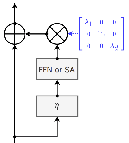
In a ViT this is applied immediately following the linear layer of the attention sublyer and the final linear layer of the feed forward sublayer. In both cases these are successive linear transforms which could be combined into one transform without loss of mathematical equivalence. At training time however this is not desirable because we wish to enforce that layer LayerScale weights are diagnolized. At inference time however, since we're not updating weights, we can multiply the LayerScale weights into linear layers' weights and biases. This is a free speed up becuase it totally eliminates the multiplication op needed to apply LayerScale.
for i in range(len(model.blocks)):
  model.blocks[i].attn.proj.weight.data.mul_(model.blocks[i].ls1.gamma.data.unsqueeze(1))
  model.blocks[i].attn.proj.bias.data.mul_(model.blocks[i].ls1.gamma.data)

  model.blocks[i].mlp.fc2.weight.data.mul_(model.blocks[i].ls2.gamma.data.unsqueeze(1))
  model.blocks[i].mlp.fc2.bias.data.mul_(model.blocks[i].ls2.gamma.data)
Footnotes
-
Oquab, M., Darcet, T., Moutakanni, T., Vo, H., Szafraniec, M., Khalidov, V., Fernandez, P., Haziza, D., Massa, F., El-Nouby, A., Assran, M., Ballas, N., Galuba, W., Howes, R., Huang, P.-Y., Li, S.-W., Misra, I., Rabbat, M., Sharma, V., Synnaeve, G., Xu, H., Jegou, H., Mairal, J., Labatut, P., Joulin, A., Bojanowski, P. DINOv2: Learning Robust Visual Features without Supervision (opens in a new tab). arXiv, 2023. ↩
-
Saying that's "all" PyTorch has to do is to put it lightly. ↩
-
Tillet, P., Kung, H.T., Cox, D. Triton: An Intermediate Language and Compiler for Tiled Neural Network Computations (opens in a new tab). MAPL, 2019. ↩
-
https://twitter.com/cHHillee/status/1786521305271157201 (opens in a new tab) ↩
-
Touvron, H., Cord, M., Sablayrolles, A., Synnaeve, G., Jégou, H. Going deeper with Image Transformers (opens in a new tab). arXiv, 2021. ↩