Transformer FLOPs
Counting the number of floating-point operations (FLOPs) in Transformers is a useful way to estimate compute requirements and measure efficiency. As training runs get larger and larger (thus more expensive) it becomes more important to understand how many FLOPs we need to do and how well we utilize our hardware.
Counting FLOPs in Transformers
One commonly used method for counting FLOPs is from the OpenAI scaling law paper 1 which uses
for estimating the number of FLOPs per token during the training of a decoder-only Transformer where is the number of non-embedding parameters in the model. To derive this we can look at the table they provide for FLOP counts of various components of the model for the forward pass.
| Operation | Parameters | FLOPs per Token |
|---|---|---|
| Embed | ||
| Attention: QKV | ||
| Attention: Mask | ||
| Attention: Project | ||
| Feedforward | ||
| De-embed | ||
| Total (Non-Embedding) |
Nonlinearities, biases, normalizations, and residuals are not counted as they turn out to be negligible. Let's explain each operation and variable here:
Embed: learned token embeddings and learned positional embeddings.- is the dimensionality of the residual stream.
Attention: QKV: linear layer in multi-head self-attention to project input into queries, keys, and values.- is the number of layers.
- is the dimensionality of the output of multi-headed attention which is equal to .
- is the dimension of the key, query, and value projections.
- is the number of attention heads in a layer.
- In practice, Transformers are implemented such that .
Attention: Mask: dot-product between query and keys.- is the context/sequence length.
Attention: Project: linear layer to project concatenated attention heads output to .Feedforward: two linear layers in the MLP block.- is the size of the output dimensionality of the first linear layer.
- is commonly used.
- is the size of the output dimensionality of the first linear layer.
De-embed: linear layer to obtain logits over vocabulary.- is the number of tokens in the vocabulary.
Combining all the non-embedding FLOPs terms gets us
for the forward pass. They note though that they drop the last term, which is context-dependent, because when it becomes negligible.
We can see this with a quick calculation using GPT-3 (, , ) as an example
which shows that the context-dependent term makes up <3% of the FLOP count. So the number of FLOPs can be simplified to just
The factor of 2 can be explained by the fact that matmuls consist of a 2 FLOP multiply-accumulate operation (one multiply and one add) for each element in a weight matrix. We can then realize that that the backward pass must account for another of FLOPs since we need to do twice the matmuls that we do during the forward pass2. This gets us to the equation.
We can then multiply by some number of tokens to estimate the total FLOPs needed for training on those tokens. Doing this we get .
Another method of calculating Transformer FLOPs is presented in DeepMind's Chinchilla scaling law paper 3. The table below shows their equations for forward pass FLOPs.
| Operation | FLOPs per Sequence |
|---|---|
| Embeddings | |
| Attention: QKV | |
| Attention: QK logits | |
| Attention: Softmax | |
| Attention: Reduction | |
| Attention: Project | |
| Feedforward | |
| Logits | |
| Total | Embeddings + (Attention + Feedforward) + Logits |
Like the first method, DeepMind also assumes the backwards pass has 2 times the FLOPs of the forward. Unlike OpenAI, DeepMind includes the FLOPs from embeddings and logits (de-embed) as well as the softmax in attention and the application of the attention pattern to the values. Also it's important to note that OpenAI's method is FLOPs per token while DeepMind's is FLOPs per sequence. This doesn't fundamentally change anything but it's important to remember in order to use either method correctly. Overall the difference between this method and tends to be pretty minimal as shown in Table A4 (Appendix F) of the Chinchilla paper.
If you want to count the FLOPs of your own transformer I've provided a FLOPs calculator app in Appendix A.
Using FLOPs to measure efficiency
Counting the number of FLOPs in our models grounds us in the reality of how much raw compute we need to run them. As training runs and models get bigger and bigger it means, of course, that training and serving these models gets more expensive. As we occupy precious resources like a A100s or H100s it becomes important to try to crunch the numbers that we need to crunch as quickly as the hardware will physically allow (emphasis on the "need" which we'll get to). To get a sense of this we will want to look at how many FLOPs/second (FLOPS, with a big S, will be used to refer to floating point operations per second and FLOPs, with a little s, is used for floating point operations with no unit of time) we execute and compare it against the theoretical peak FLOPS of our hardware. In practice, we'll never be able to achieve that peak, but it's useful to know how far away we are from it.
One method that can be used for measuring training efficiency is hardware FLOPS utilization (HFU). This approach is the ratio of all FLOPs we execute per second to the theoretical peak FLOPS. This would take into account all the FLOPs we estimate for a regular forward+backward pass, but also redundant computation we need to do in order to train large models on the current hardware like rematerialization for activation checkpointing4. While this method of measurement can be useful, the inclusion of computation like rematerilization can make it seem like our training is more efficient than it really is. Ultimately, if we could train these models without tricks like activation checkpointing we would. It's only there as a work around due to constraints of current hardware and being able to eliminate it one day would be efficient. What we really care about is only the FLOPs we need to do to train the model in theory which is just the forward+backward FLOPs, or the model FLOPs.
The best practice now for reporting LLM training efficiency is known as model FLOPs utilization (MFU) which was proposed in Google's PaLM paper5. The idea is to focus on how efficiently we executed just the necessary model FLOPs. The calculation is quite simple as all we need to do is multiply our FLOPs count by the observed throughput (tokens/sequences per second), and then divide by the theoretical peak FLOPS of our hardware.
where is the model's FLOPs per token, is the observed tokens per second, and is the theoretical peak FLOPS.
For example, when using the fp16/bf16 formats an A100 has a theoretical peak of 312 teraFLOPS (TFLOPS)6. If we use the estimate for forward+backward FLOPs and are training a 125M parameter model using an A100 and we have throughput of 200,000 tokens per second then our MFU is
Which means we achieved 48% of the theoretical peak FLOPS. With this method if we are doing something like activation checkpointing this will hurt our MFU, but it wouldn't necessarily hurt our HFU. Conversely, if we could get away with not using activation checkpointing then our MFU would improve. This isn't to say HFU is worthless though. If we need to use activation checkpointing, HFU can help gauge the efficiency of our rematerilization implementation. In the long run though we should generally want to optimize for MFU and it also allows fairer comparison of efficiency across different training set ups.
In practice, the range of MFU for language models can vary widely depending on model size, hardware7, and implementation details, but generally range between 10-65%8 9 10.
Scaling of FLOPs
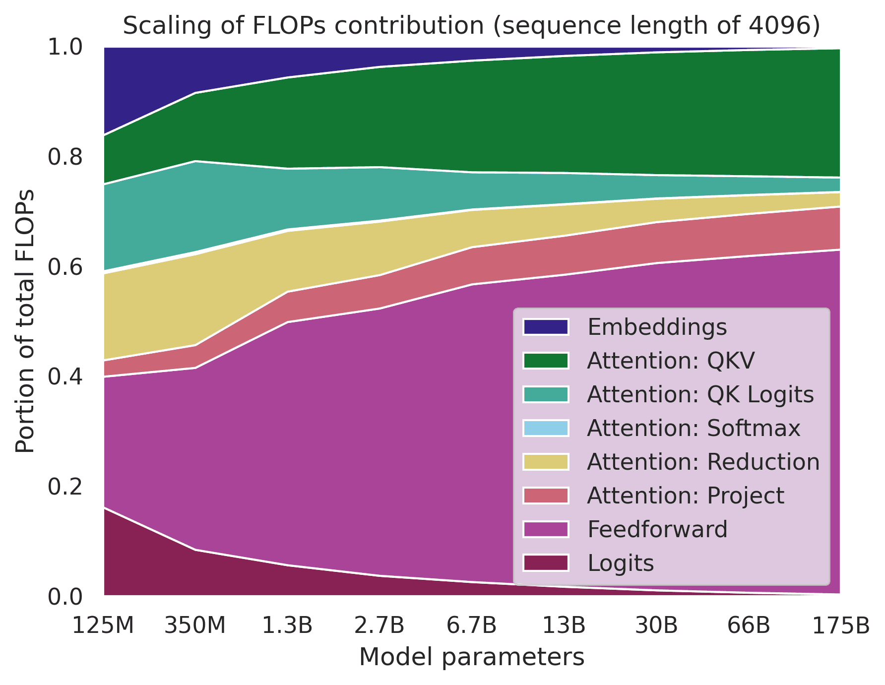
As we scale the size of Transformers it can be useful to know how different components of the model contribute to the computational cost11 12 13. Let's look at how the FLOPs of these components (using the operations in the DeepMind table) contribute to the total compute as we scale the model.

The plot above shows this evolution using the GPT-314/OPT15 model family (with a sequence length of 4096). As we can see, the Embeddings and Logits become a very miniscule portion of FLOPs while the matmuls of the linear layers in Attention: QKV and Feedforward become dominant.
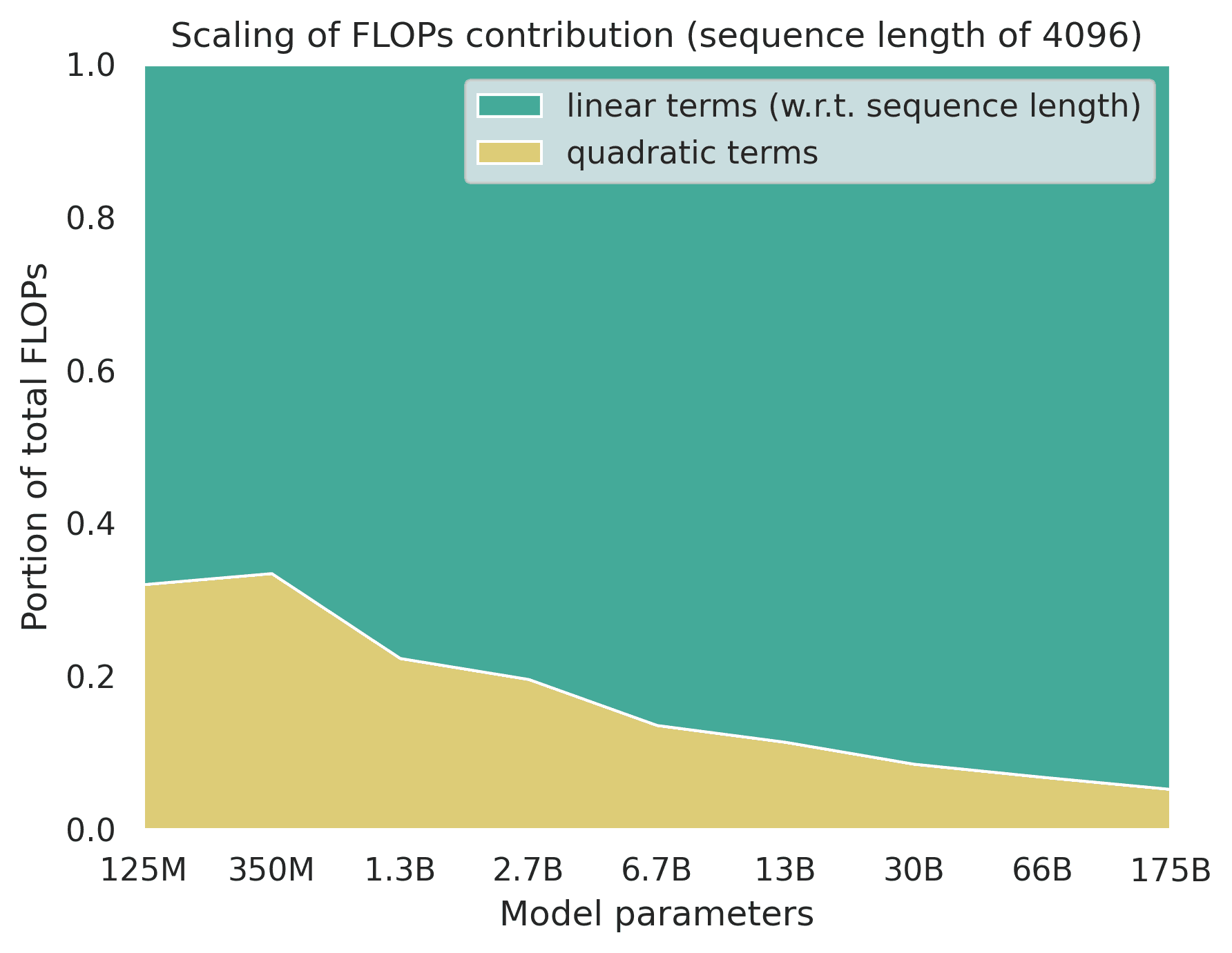
A useful way to look at this is to divide the components of the model into two buckets: terms that scale linearly with sequence length and those that scale quadratically. The terms that scale quadratically with sequence length are Attention: QK logits, Attention: Softmax, and Attention: Reduction. All other terms (Embeddings, Attention: QKV, Attention: Project, Feedforward and Logits) scale linearly with sequence length.
We can calculate FLOPs for various model sizes and look at how these terms evolve as the number of parameters increases.

For the smallest models the quadratic attention terms make up over 30% of the FLOPs, but this steadily decreases. Somewhere between 13B and 30B it starts to account for <10% of FLOPs. The dominance of the "linear" terms is explained by the fact that the size of the weight matrices in linear layers does scale quadratically but with respect to . So by making our model wider we know that we'll be increasing the portion of FLOPs that come from the linear layers.
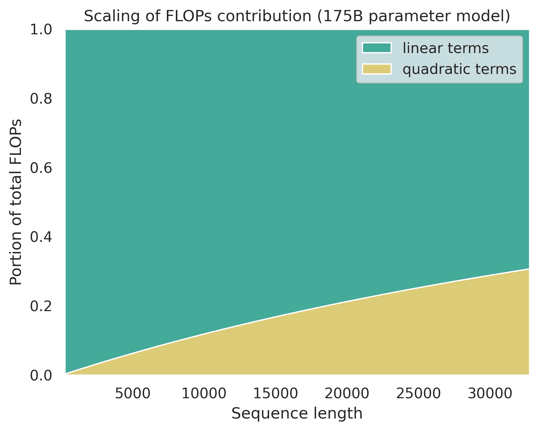
We can also look at the scaling of these components from the view of a fixed model size but varying sequence length.

This shows for a 175B parameter model how much the quadratic terms contribute to total FLOPs as sequence length scales. For the smallest sequence lengths (i.e. 256 or 512) the quadratic terms make up <1% of FLOPs. After the 8192 mark they then make up >10% and then hit 31% for a 32K length sequence.
So at large scales the quadratic nature of attention only makes up a fraction of the model's FLOPs even at longer sequence lengths.
Although the scope of this post is FLOPs bound (pun intended), when it comes to profiling and optimizing models there is much more to consider. Here are some helpful resources to read more in that direction:
- Transformer Inference Arithmetic (opens in a new tab)
- Making Deep Learning Go Brrrr From First Principles (opens in a new tab)
- Data Movement Is All You Need: A Case Study on Optimizing Transformers (opens in a new tab)
Citation
@article{casson2023transformerflops,
  author={Adam Casson},
  title={Transformer FLOPs},
  year={2023},
  url={https://adamcasson.com/posts/transformer-flops}
}
A PDF version of this post can be found here (opens in a new tab).
Appendix A: Transformer FLOPs calculator
View the source code for this app here (opens in a new tab).
Appendix B: FLOPs counting methods in code
OpenAI's counting method in code:
def openai_flops_per_token(n_layers, n_heads, d_model, n_ctx, n_vocab, ff_ratio=4):
    """Open AI method for forward pass FLOPs counting of decoder-only Transformer
    """
    d_attn = d_model // n_heads
    d_ff = d_model * ff_ratio

    embeddings = 4 * d_model
    attn_qkv = 2 * n_layers * d_model * 3 * (d_attn * n_heads)
    attn_mask = 2 * n_layers * n_ctx * (d_attn * n_heads)
    attn_project = 2 * n_layers * (d_attn * n_heads) * d_model
    ff = 2 * n_layers * 2 * d_model * d_ff
    logits = 2 * d_model * n_vocab

    return embeddings + attn_qkv + attn_mask + attn_project + ff + logits
DeepMind's counting method in code:
def deepmind_flops_per_sequence(n_layers, n_heads, d_model, n_ctx, n_vocab, ff_ratio=4):
    """DeepMind method for forwad pass FLOPs counting of decoder-only Transformer
    """
    d_attn = d_model // n_heads
    d_ff = d_model * ff_ratio

    embeddings = 2 * n_ctx * n_vocab * d_model

    attn_qkv = 2 * n_ctx * 3 * d_model * (d_attn * n_heads)
    attn_logits = 2 * n_ctx * n_ctx * (d_attn * n_heads)
    attn_softmax = 3 * n_heads * n_ctx * n_ctx
    attn_reduce = 2 * n_ctx * n_ctx * (d_attn * n_heads)
    attn_project = 2 * n_ctx * (d_attn * n_heads) * d_model
    total_attn = attn_qkv + attn_logits + attn_softmax + attn_reduce + attn_project

    ff = 2 * n_ctx * (d_model * d_ff + d_model * d_ff)

    logits = 2 * n_ctx * d_model * n_vocab

    return embeddings + n_layers * (total_attn + ff) + logits
Appendix C: FLOPs counting in Vision Transformer (ViT)
Extending these methods to a standard ViT is straight forward and the main difference we have to account for is the patch embeddings and logits (highlighted below). Using the DeepMind method for FLOPs counting, we can modify it as such for a ViT with a classification head:
| Operation | FLOPs per Image |
|---|---|
| Embeddings | |
| Attention: QKV | |
| Attention: QK logits | |
| Attention: Softmax | |
| Attention: Reduction | |
| Attention: Project | |
| Feedforward | |
| Logits | |
| Total | Embeddings + (Attention + Feedforward) + Logits |
- is the number of patches in our image.
- is the length of the side of a patch in pixels.
- i.e. means one patch is of size .
- is the number of channels in the input image.
- to account for the prepending of a learnable [CLS] token.
Logitsis a linear layer for predicting using a single token as input (i.e. the [CLS] token, mean pool of image tokens, etc.).
For example, if our input image is an RGB image of size and we have non-overlapping patches of size then and .
Since the patch embedding layer is applied to non-overlapping patches, we can also easily express it in terms of the total number of pixels in the image
Footnotes
-
Kaplan, J., McCandlish, S., Henighan, T., Brown, T.B., Chess, B., Child, R., Gray, S., Radford, A., Wu, J., Amodei, D. Scaling Laws for Neural Language Models (opens in a new tab). arXiv, 2020. ↩
-
Bahdanau, D., The FLOPs Calculus of Language Model Training (opens in a new tab). See section Derivation of Transformer FLOPs Equation for a good explanation of each forward+backward FLOP for a single weight. 2022. ↩
-
Hoffmann, J., Borgeaud, S., Mensch, A., Buchatskaya, E., Cai, T., Rutherford, E., de Las Casas, D., Hendricks, L.A., Welbl, J., Clark, A., Hennigan, T., Noland, E., Millican, K., van den Driessche, G., Damoc, B., Guy, A., Osindero, S., Simonyan, K., Elsen, E., Rae, J.W., Vinyals, O., Sifre, L. Training Compute-Optimal Large Language Models (opens in a new tab). arXiv, 2022. ↩
-
If we can't store activations in memory then we can do activation checkpointing by throwing out the activations after they aren't needed anymore in the forward pass and then re-computing (a.k.a rematerializing) them during the backward pass. If done for all activations this would amount to an extra forward pass and thus our would increase to . ↩
-
Chowdhery, A., Narang, S., Devlin, J., Bosma, M., Mishra, G., Roberts, A., Barham, P., Chung, H.W., Sutton, C., Gehrmann, S., Schuh, P., Shi, K., Tsvyashchenko, S., Maynez, J., Rao, A., Barnes, P., Tay, Y., Shazeer, N., Prabhakaran, V., Reif, E., Du, N., Hutchinson, B., Pope, R., Bradbury, J., Austin, J., Isard, M., Gur-Ari, G., Yin, P., Duke, T., Levskaya, A., Ghemawat, S., Dev, S., Michalewski, H., Garcia, X., Misra, V., Robinson, K., Fedus, L., Zhou, D., Ippolito, D., Luan, D., Lim, H., Zoph, B., Spiridonov, A., Sepassi, R., Dohan, D., Agrawal, S., Omernick, M., Dai, A.M., Pillai, T.S., Pellat, M., Lewkowycz, A., Moreira, E., Child, R., Polozov, O., Lee, K., Zhou, Z., Wang, X., Saeta, B., Diaz, M., Firat, O., Catasta, M., Wei, J., Meier-Hellstern, K., Eck, D., Dean, J., Petrov, S., Fiedel, N. PaLM: Scaling Language Modeling with Pathways (opens in a new tab). arxiv, 2022. ↩
-
Although MFU normalizes according to a hardware's theoretical peak FLOPs there can be many factors that impact this including memory-bandwidth, cross-device/cross-node communication bandwidth, etc. ↩
-
MosaicML. MosaicBERT: Pretraining BERT from Scratch for $20 (opens in a new tab). See section Multinode Scaling of MosaicBERT. 2023. ↩
-
MosaicML. MosaicGPT Training Benchmarks (opens in a new tab). 2023. ↩
-
Roller, S. Twitter (opens in a new tab). 2022. ↩
-
He, H., Twitter (opens in a new tab). 2022. ↩
-
Timbers, F. Twitter (opens in a new tab). 2023. ↩
-
Brown, T.B., Mann, B., Ryder, N., Subbiah, M., Kaplan, J., Dhariwal, P., Neelakantan, A., Shyam, P., Sastry, G., Askell, A., Agarwal, S., Herbert-Voss, A., Krueger, G., Henighan, T., Child, R., Ramesh, A., Ziegler, D.M., Wu, J., Winter, C., Hesse, C., Chen, M., Sigler, E., Litwin, M., Gray, S., Chess, B., Clark, J., Berner, C., McCandlish, S., Radford, A., Sutskever, I., Amodei, D. Language Models are Few-Shot Learners (opens in a new tab). arxiv, 2022. ↩
-
Zhang, S., Roller, S., Goyal, N., Artetxe, M., Chen, M., Chen, S., Dewan, C., Diab, M., Li, X., Lin, X.V., Mihaylov, T., Ott, M., Shleifer, K., Simig, D., Koura, P.S., Sridhar, A., Wang, T., Zettlemoyer, L. OPT: Open Pre-trained Transformer Language Models (opens in a new tab). arxiv, 2022. ↩